In hydraulic design it is common to encounter implicit equations that cannot be directly solved. Traditionally these were solved in an iterative manner, where an initial guess is refined until convergence of the solution is achieved. With programmable calculators becoming common in the late 20th century, and computers and smartphones providing even more convenient computation capacity in the 21st century, the need for graphical aids and lengthy iterative procedures has become largely obsolete. However, these iterative methods underlie many advanced tools, and having a level of comfort with them can allow the development of custom tools to solve other unique problems.
Illustrated below are examples of solving hydraulic equations using a variety of methods. Most of these examples use R, though an example using a spreadsheet is also included. Similar approaches to those used here are available in other languages, like Matlab and python.
1.0 An Example with Flow in a Pipe Under Pressure
As water flows through a pipe energy is lost due to friction with the pipe walls and local disturbances (minor losses). For this example assume minor losses are negligible. The energy head loss due to friction with the walls of the pipe is described by the Darcy-Weisbach equation, which estimates the energy loss per unit weight, or head loss hf, which has units of length. For circular pipes it is expressed as: \[h_f = \frac{fL}{D}\frac{V^2}{2g} = \frac{8fL}{\pi^{2}gD^{5}}Q^{2}\] In this equation f is the friction factor, most accurately calculated with the Colebrook equation: \[\frac{1}{\sqrt{f}} = -2\log\left(\frac{\frac{k_s}{D}}{3.7} + \frac{2.51}{Re\sqrt{f}}\right)\] where ks is the absolute roughness of the pipe wall. The Reynolds number, \(Re=\frac{VD}{\nu}\) describes the turbulence of the flow. The Colebrook equation is commonly plotted as a Moody diagram to illustrate the relationships between the variables:
library(hydraulics)
moody()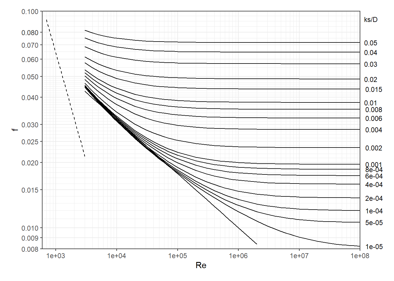
1.1 Solving for Head Loss by Manual Iteration
The simplest pipe flow problem to solve is when the unknown is head loss, hf, since all variables on the right side of the Darcy-Weisbach equation are known, except f. For this example, we will find the head loss (due to friction) of 20oC water in a pipe with the following characteristics: Q=0.416 m3/s, L=100m, D=0.5m, ks=0.046mm.
Since the water temperature is known, first find the kinematic viscocity of water, \({\nu}\), since it is needed for the Reynolds number. This can be obtained from a table in a reference or using software. Here we will use the hydraulics R package.
nu <- kvisc(T=20, units="SI")
cat(sprintf("Kinematic viscosity = %.3e m2/s\n", nu))
## Kinematic viscosity = 1.023e-06 m2/sWe will need the Reynolds Number to use the Colebrook equation, and that can be calculated since Q is known. This can be accomplished with a calculator, or using other software (R is used here):
Q <- 0.416
D <- 0.5
A <- (3.14/4)*D^2
V <- Q/A
Re <- V*D/nu
cat(sprintf("Velocity = %.3f m/s, Re = %.3e\n", V, Re))
## Velocity = 2.120 m/s, Re = 1.036e+06Now the only unknown in the Colebrook equation is f, but unfortunately f appears on both sides of the equation.
To begin the iterative process, a first guess at f is needed. A reasonable value to use is the minimum f value, fmin, given the known \(\frac{k_s}{D}=\frac{0.046}{500}=0.000092=9.2\cdot 10^{-5}\). Reading horizontally from the right vertical axis to the left on the Moody diagram provides a value for \(f_{min}\approx 0.012\). In addition, it can be seen that f is independent of Re for large values of Re. When Re is large the Colebrook equation approaches: \[\frac{1}{\sqrt{f}} = -2\log\left(\frac{\frac{k_s}{D}}{3.7}\right)\] Using this the same value of fmin=0.012 is obtained.
Iteration 1: Using f=0.012 the right side of the Colebrook equation is 8.656. the next estimate for f is then obtained by \(\frac{1}{\sqrt{f}}=8.656\) so f=0.0133.
Iteration 2: Using the new value of f=0.0133 in the right side of the Colebrook equation produces 8.677. A new value for f is obtained by \(\frac{1}{\sqrt{f}}=8.677\) so f=0.0133. The solution has converged!
Using the new value of f, the value for hf is calculated: \[h_f = \frac{8fL}{\pi^{2}gD^{5}}Q^{2}=\frac{8(0.0133)(100)}{\pi^{2}(9.81)(0.5)^{5}}(0.416)^{2}=0.061 m\]
1.2 Solving for head loss using an equation solver
First, rearrange the Colebrook equation so all terms are on one side of the equation: \[-2\log\left(\frac{\frac{k_s}{D}}{3.7} + \frac{2.51}{Re\sqrt{f}}\right) - \frac{1}{\sqrt{f}}=0\] Create a function using whatever equation solving platform you prefer. Here the R software is used:
colebrk <- function(f,ks,D,Re) -2.0*log10((ks/D)/3.7 + 2.51/(Re*(f^0.5)))-1/(f^0.5)Find the root of the function (where it equals zero), specifying a reasonable range for f values using the interval argument:
f <- uniroot(colebrk, interval = c(0.008,0.1), ks=0.000046, D=0.5, Re=1.036e+06)$root
cat(sprintf("f = %.4f\n", f))
## f = 0.0133The same value for hf as above results.
1.3 Solving for Q Using Manual Iteration
For this example, we wish to find the flow rate, Q of 20oC water in a pipe with the following characteristics: hf=0.6m, L=100m, D=0.5m, ks=0.046mm.
First rearrange the Darcy-Weisbach equation to express V as a function of f, substituting all of the known quantities: \[V = \sqrt{\frac{h_f}{L}\frac{2gD}{f}}=\frac{0.243}{\sqrt{f}}\]
That provides one equation relating V and f. The second equation relating the two is one of the friction factor equations, such as the Colebrook equation or its graphic representation in the Moody diagram. An initial guess at a value for f is obtained using fmin=0.012 as was done above.
Iteration 1: \(V=\frac{0.243}{\sqrt{0.012}}=2.218\); \(Re=\frac{2.218\cdot 0.5}{1.023e-06}=1.084 \cdot 10^6\). A new f value is obtained from the Moody diagram or an equation using the new Re value: \(f \approx 0.0131\)
Iteration 2: \(V=\frac{0.243}{\sqrt{0.0131}}=2.123\); \(Re=\frac{2.123\cdot 0.5}{1.023e-06}=1.038 \cdot 10^6\). A new f estimate: \(f \approx 0.0132\)
The function converges very quickly if a reasonable first guess is made. Using V=2.12 m/s, \(Q = AV = \left(\frac{\pi}{4}\right)D^2V=0.416 m^3/s\)
1.4 Solving for Q Using an Explicit Equation
Solving the Darcy Weisbach equation for \(\frac{1}{\sqrt{f}}\) and substituting that into the Colebrook equation produces:\[Q=-2.221D^2\sqrt{\frac{gDh_f}{L}} \log\left(\frac{\frac{k_s}{D}}{3.7} + \frac{1.784\nu}{D}\sqrt{\frac{L}{gDh_f}}\right)\] This can be solved explicitly for Q=0.413 m3/s.
1.5 Solving for Q Using an R package
Using software to solve the problem allows the use of the Colebrook equation in a straightforward format. The hydraulics package in R is applied to the same problem as above.
ans <- darcyweisbach(D=0.5, hf=0.6, L=100, ks=0.000046, nu=1.023e-06, units = c('SI'))
knitr::kable(format(as.data.frame(ans), digits = 3), format = "pipe")| Q | V | L | D | hf | f | ks | Re |
|---|---|---|---|---|---|---|---|
| 0.406 | 2.07 | 100 | 0.5 | 0.6 | 0.0133 | 4.6e-05 | 1010392 |
The answer differs from the manual iteration by just over 2%, showing remarkable consistency.
1.6 Solving for D using manual iterations
If we use Q=0.416m3/s and solve for D, iterative solutions become very cumbersome since neither V (hence Re), nor ks/D are known. It can, however, be done. Rearranging the equation from section 1.4 above allows this to be solved for zero, which can be done manually by guessing values and repeating the calculation in a spreadsheet or with a tool like R. \[-2.221D^2\sqrt{\frac{gDh_f}{L}} \log\left(\frac{\frac{k_s}{D}}{3.7} + \frac{1.784\nu}{D}\sqrt{\frac{L}{gDh_f}}\right)-Q=0\] Iteration 1: Guess an arbitrary value of D=0.3m. Solve the left side of the equation to obtain a value of -0.31
Iteration 2: Guess another value for D=1.0m, which produces a value for the function of 2.11
The root, when the function equals zero, lies between the two values,
so the correct D is between 0.3 and 1.0. Repeated values can home in on
a solution. Plotting the results from many trials can help guide toward
the solution.
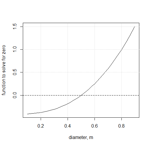 The root is seen to lie very close to D=0.5 m.
1.7 Solving for D using an equation solver
An equation solver automatically accomplishes the manual steps of the prior demonstration. The equation from 1.6 can be written as a function that can then be solved for the root, again using R software for the demonstration:
q_fcn <- function(D, Q, hf, L, ks, nu, g) {
  -2.221 * D^2 * sqrt(( g * D * hf)/L) * log10((ks/D)/3.7 + (1.784 * nu/D) * sqrt(L/(g * D * hf))) - Q
}
The uniroot function can solve the equation in R (or use a comparable approach in other software) for a reasonable range of D values
ans <- uniroot(q_fcn, interval=c(0.01,4.0),Q=0.416, hf=0.6, L=100, ks=0.000046, nu=1.023053e-06, g=9.81)$root
cat(sprintf("D = %.3f m\n", ans))
## D = 0.501 m2.0 An Example with Uniform Open channel Flow
The Manning equation describes flow conditions in an open channel under uniform flow conditions. It is often expressed as: \[Q=A\frac{C}{n}{R}^{\frac{2}{3}}{S}^{\frac{1}{2}}\] where C is 1.0 for SI units and 1.49 for Eng (U.S. Customary) units. Q is the flow rate, A is the cross-sectional flow area, n is the Manning roughness coefficient, S is the longitudinal channel slope, and R is the hydraulic radius \(R=\frac{A}{P}\), where P is the wetted perimeter.
In engineering applications one of the most common channel shapes is trapezoidal.
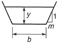
For a trapezoid the relationships for area and wetted perimeter are: \(A=(b+my)y\) and \(P=b+2y\sqrt{1+m^2}\). Substituting these into Manning’s equation produces:
\[Q=\frac{C}{n}{\frac{\left(by+my^2\right)^{\frac{5}{3}}}{\left(b+2y\sqrt{1+m^2}\right)^\frac{2}{3}}}{S}^{\frac{1}{2}}\] Rearranging to a form of y(x) = 0 allows the use of a standard solver to find the root(s):
\[Q-\frac{C}{n}{\frac{\left(by+my^2\right)^{\frac{5}{3}}}{\left(b+2y\sqrt{1+m^2}\right)^\frac{2}{3}}}{S}^{\frac{1}{2}}=0\]
2.1 Using an Equation Solver in R
R is a powerful open-source (free) programming language, and can be used along with an excellent interface RStudio for technical analysis. By installing these, you can access functions to solve equations.
In R, the Mannning equation can be set up as a function in terms of a missing variable, here using normal depth, y as the missing variable.
yfun <- function(y) {
  Q - (((y * (b + m * y)) ^ (5 / 3) * sqrt(S)) * (C / n) / ((b + 2 * y * sqrt(1 + m ^ 2)) ^ (2 / 3)))
  }
As an example of solving for y when given other input variables, first define the known input. In this example Q=225 ft3/s, n=0.016, m=2, b=10 ft, S=0.0006, and because these use US Customary (or English) units, C=1.486.
Q <- 225.
n <- 0.016
m <- 2
b <- 10.0
S <- 0.0006
C <- 1.486
While not necessary, a plot can be instructive as far as what to expect for a solution.
ys <- seq(0.1, 5, 0.1)
plot(ys,yfun(ys), type='l', xlab = "y, ft", ylab = "Function to solve for zero")
abline(h=0)
grid()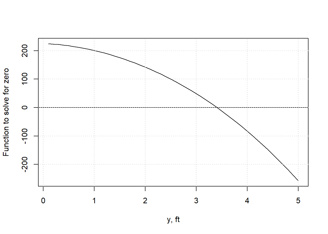
This plot indicates that the solution, when the function has a value of 0, should occur for a depth, y of something a little less than 3.5.
The R function uniroot can be used to find a single root within a defined interval.
ans <- uniroot(yfun, interval = c(0.0000001, 200), extendInt = "yes")
cat(sprintf("Normal Depth: %.3f ft\n", ans$root))
## Normal Depth: 3.406 ftIf you need to solve an equation with multiple roots, the rootSolve package has a uniroot.all function.
2.2 Using a pre-built R package
There is a hydraulics package for R that has built-in functions to solve many hydraulics problems. You can install it in R and load it.
library(hydraulics)The hydraulics package has a manningt function for trapezoidal channels. Specifying “Eng” units ensures the correct C value is used. Sf is the same as S above.
ans <- manningt(Q = 225., n = 0.016, m = 2, b = 10., Sf = 0.0006, units = "Eng")
cat(sprintf("Normal Depth: %.3f ft\n", ans$y))
## Normal Depth: 3.406 ft2.3 Using a Spreadsheet Like Excel
Spreadsheet software is very popular and has been modified to be able to accomplish many technical tasks such as solving equations. This example uses Excel with its solver add-in activated, though other spreadsheet software has similar solver add-ins that can be used.
The first step is to enter the input data along with an initial guess for the variable you wish to solve for. The equation for which a root will be determined is typed in using the initial guess for y in this case.
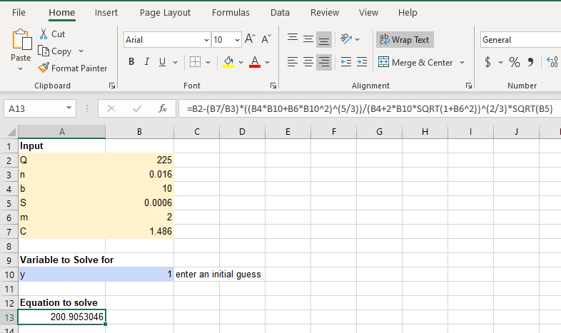
At this point you could use a trial-and-error approach and simply try different values for y until the equation produces something close to 0.
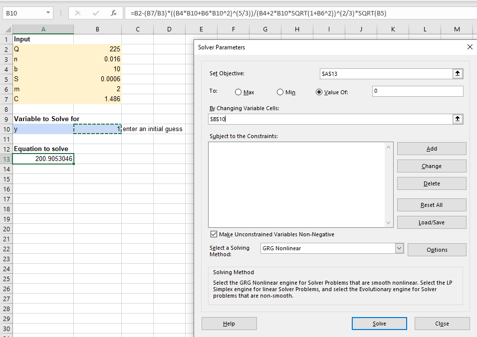
A more efficient method is to use a solver. Check that the solver add-in is activated (in Options) and open it. Set the values appropriately.
Click Solve and the y value that produces a zero for the
equation will appear.
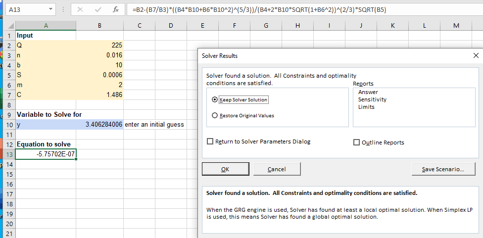
If you need to solve for multiple roots, you will need to start from different initial guesses.
3.0 Solving a System of Equations
In the examples above the challenge was often to solve a single implicit equation. The manual iteration approach can work to solve two equations, but as the number of equations increases, especially when using implicit equations, using an equation solver is needed.
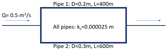
For the case of a simple pipe loop manual iterations are impractical.
This example uses a single loop, essentially a parallel pipe problem.
 The fundamental equations needed are the Darcy-Weisbach equation, the
Colebrook equation, and continuity (conservation of mass). For the
illustrated system, this means:
The fundamental equations needed are the Darcy-Weisbach equation, the
Colebrook equation, and continuity (conservation of mass). For the
illustrated system, this means:
- The flows through each pipe must add to the total flow
- The head loss through Pipe 1 must equal that of Pipe 2
This could be set up as a system of anywhere from 2 to 10 equations to solve simultaneously. In this example four equations are used: \[Q_1+Q_2-Q_{total}=V_1\frac{\pi}{4}D_1^2+V_2\frac{\pi}{4}D_2^2-0.5m^3/s=0\] \[h_{f1}-h_{f2} = \frac{f_1L_1}{D_1}\frac{V_1^2}{2g} -\frac{f_2L_2}{D_2}\frac{V_2^2}{2g}=0\] Two additional equations are the Colebrook equation for solving for friction factor, as in Section 1.2 above. These four equations can be solved simultaneously using an equation solver, such as the fsolve function in the R package pracma.
library(pracma)
library(hydraulics)

#assign known inputs - SI units
Qsum <- 0.5
D1 <- 0.2
D2 <- 0.3
L1 <- 400
L2 <- 600
ks <- 0.000025
g <- 9.81
nu <- kvisc(T=100, units='SI')

#Set up the function that sets up 4 unknowns (x) and 4 equations (y)
F_trial <- function(x) {
  V1 <- x[1]
  V2 <- x[2]
  f1 <- x[3]
  f2 <- x[4]
  Re1 <- V1*D1/nu
  Re2 <- V2*D2/nu
  y <- numeric(length(x))
  #Continuity - flows in each branch must add to total
  y[1] <- V1*pi/4*D1^2 + V2*pi/4*D2^2 - Qsum
  #Darcy-Weisbach equation for head loss - must be equal in each branch
  y[2] <- f1*L1*V1^2/(D1*2*g) - f2*L2*V2^2/(D2*2*g)
  #Colebrook equation for friction factors
  y[3] <- -2.0*log10((ks/D1)/3.7 + 2.51/(Re1*(f1^0.5)))-1/(f1^0.5)
  y[4] <- -2.0*log10((ks/D2)/3.7 + 2.51/(Re2*(f2^0.5)))-1/(f2^0.5)
  return(y)
}

#provide initial guesses for unknowns and run the fsolve command
xstart <- c(2.0, 2.0, 0.01, 0.01)
z <- fsolve(F_trial, xstart)

#prepare some results to print
Q1 <- z$x[1]*pi/4*D1^2
Q2 <- z$x[2]*pi/4*D2^2
hf1 <- z$x[3]*L1*z$x[1]^2/(D1*2*g)
hf2 <- z$x[4]*L2*z$x[2]^2/(D2*2*g)
cat(sprintf("Q1=%.2f, Q2=%.2f, V1=%.1f, V2=%.1f, hf1=%.1f, hf2=%.1f, f1=%.3f, f2=%.3f\n", Q1,Q2,z$x[1],z$x[2],hf1,hf2,z$x[3],z$x[4]))
## Q1=0.15, Q2=0.35, V1=4.8, V2=5.0, hf1=30.0, hf2=30.0, f1=0.013, f2=0.012If the fsolve command fails, a simple solution is sometimes to revise your initial guesses and try again. There are other solvers in R and every other scripting language that can be similarly implemented (For example, both python and MatLab also have an fsolve function).
 This work is licensed under a Creative Commons Attribution 4.0 International License.